A. Chi-Square Goodness of Fit

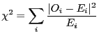
To determine the quality of the fits, we bin the scores and calculate the $\chi^2$ statistic

$$\chi^2 = \sum_i \frac{ \vert O_i - E_i\vert^2}{E_i}$$ (17)

where $O_i$ and $E_i$ are the observed and expected frequencies respectively for bin $i$ . The expected frequency is calculated by

$$E_i = t\, (F(s_{i,a}) - F(s_{i,b}))$$

where $s_{i,a}$ and $s_{i,b}$ are respectively the lower and upper score limits of bin $i$ , and $F(s) = (1-G_t) F(s\vert) + G_t F(s\vert 1)$ is the cumulative distribution function of the mixture under estimation.

The statistic follows, approximately, a $\chi^2$ distribution with $M-4-1$ degrees of freedom, where $M$ is the number of bins and $4$ is the number of parameters we estimate. The null hypothesis $\mathrm{H}_0$ is that the observed data follow the estimated mixture. $\mathrm{H}_0$ is rejected if the $\chi^2$ of the fit is above the critical value of the corresponding $\chi^2$ distribution at a significance level of 0.05 [15].

For the $\chi^2$ approximation to be valid, $E_i$ should be at least 5, thus we may combine bins in the right tail when $E_i < 5$ . When the last $E_i$ does not reach 5 even for $b=+\infty$ , we only then apply the Yates' correction, i.e. subtract 0.5 from the absolute difference of the frequencies in Equation 17 before squaring.

Different fits on the same data can result to slightly different degrees of freedom due to combining bins. To compare the quality of different fits, so we can keep track of the best one irrespective its $\mathrm{H}_0$ status, we use the $\chi^2$ upper-probability; the higher the probability, the better the fit. As an initial upper-probability reference, we use the one of an exponential-only fit, produced by setting $\lambda = 1/(\mu_s-s_t)$ .

The $\chi^2$ statistic is sensitive to the choice of bins.

A..1 Score Binning

For binning, we use the optimal number of bins as this is given by the method described in [12]. The method considers the histogram to be a piecewise-constant model of the underlying probability density. Then, it computes the posterior probability of the number of bins for a given data set. This enables one to objectively select an optimal piecewise-constant model describing the density function from which the data were sampled. For practical reasons, we cap the number of bins to a maximum of 200.