5. Experimental Results and Discussion

Table 1 summarizes the average precision results of all experiments and their percentage change with respect to the baseline of Sw the traditional indexing approach.

 

Table 1: Average precision results

	small topics		large topics
run	av. prec.	change	av. prec.	change
w	0.525	-2.2%	0.696	+0.4%
Sw	0.537	baseline	0.693	baseline
Lw	0.547	+1.9%	0.693	0.0%
Ln	0.559	+4.1%	0.678	-2.2%
Lnj	0.563	+4.8%	0.695	+0.3%
Lnv	0.540	+0.5%	0.683	-1.4%
Lnjv	0.548	+2.0%	0.694	+0.1%
Lnj+Lap	0.633	+17.9%	0.730	+5.3%
Lnj+Lbt	0.620	+15.4%	0.732	+5.6%

5.1 Stemming vs. Lemmatization

The experiments with unstemmed, stemmed and lemmatized words (w, Sw and Lw) as index terms showed no significant differences in average precision ($<5.0\%$). That was not expected, since it is well-known that stemming improves performance in retrieval environments. However, this does not seem to be the case in classification environments. Classifiers can been seen as long queries. While retrieval queries contain usually 2-3 keywords, the average length of our classifiers for these experiments were 28.9, 26.1, and 26.1 keywords respectively. An automated method for building classifiers like Rocchio's, given sufficient training data, will identify and include all potential morphological variants of significant keywords into a classifier. That makes any form of morphological normalization in such environments redundant. Nevertheless, when no sufficient training data are available (like for the small topics), differences in performance grow larger. In this case, lemmatization is slightly better than stemming which is slightly better than no stemming at all.

The results suggest that for short queries (like in text retrieval), or for insufficient training data (like at the beginning of a text filtering task), morphological normalization will be useful, and lemmatization will be more beneficial for effectiveness than stemming since it is less error-prone. For long and precise queries (like classification queries derived from sufficient training data), morphological normalization has no significant impact on effectiveness. In any case, morphological normalization reduces the number of terms an information seeking system has to deal with, so it can always be used as a feature reduction mechanism.

5.2 Part-Of-Speech-based Indexing

The experiments based on indexing sets derived from combinations of part-of-speech categories (Ln, Lnj, Lnv, and Lnjv) presented, as well, no significant improvements over the baseline of stemmed words. Of course, all these experiments included, at least, the category of nouns. When we tried to exclude nouns, performance degraded greatly, confirming the importance of nouns for indexing.

If we were allowed to draw a weak conclusion from these results, we could have said that the union of nouns and adjectives (Lnj) performs best, while the addition of verbs reduces performance, and adverbs do not make a difference (we should remind that the difference between the indexing sets Lnjv and Lw is that the former does not include adverbs). The poor performance of verbs may be related to a limited or poor usage of them in the Reuters data, or to some bad interaction between between nouns and verbs. A confusion between nouns and verb arises from the fact most nouns can be verbed (e.g. verb $\to$ verbed) and verbs can be nominalized (e.g. to visit $\to$ a visit). This issue requires a further investigation.

Despite the non-significant differences in average precision, part-of-speech information may be used to assist term selection mechanisms, like morphological normalization may do. Table 2 gives a comparison of the number of distinct terms our system had to deal with in different experiments.

 

Table 2: Distinct term occurrences

run	distinct terms	reduction
w	34030	baseline
Sw	27205	20.0%
Lw	29377	13.7%
Ln	23039	32.3%
Lnj	26952	20.8%
Lnv	24997	26.5%
Lnjv	28804	15.3%

It can be seen that the lemmatized union of nouns and adjectives Lnj consists of 20.8% less indexing terms than the indexing set of all keywords w, while it preserves the effectiveness (it actually even improves it). Such a POS-based feature reduction mechanism has already been seen in [14] where nouns and adjectives were assumed to be most vital in representing document contents, but no comparative empirical evaluation was given.

5.3 Composite Indexing Terms

Since the best performance was presented by Lnj, we decided to add to this run composite terms in the form of adjacent pairs Lnj+Lap, or binary terms Lnj+Lbt.

Both experiments led to significant improvements ($>5.0\%$) in average precision. Considering Lnj as the baseline, the improvement was 12.4% (small topics) and 5.0% (large topics) for adjacent pairs, and 10.1% (small topics) and 5.3% (large topics) for binary terms. Figure 2 gives the 11-point interpolated recall-precision curves.

  

Figure 2: The impact of adding composite terms to the indexing set of nouns and adjectives

We did not use a special weighting scheme for composite terms. Composite terms were simply mixed up with single terms and weighted using the same ltc weighting formula (equation 2). This clearly violates the term independence assumption of the vector space model. In order to compensate for this, when single and composite (phrasal) terms are indexed together, composite terms are traditionally weighted lower [6], something we did not do. This suggests that there is margin for even better performance assuming a proper weighting scheme.

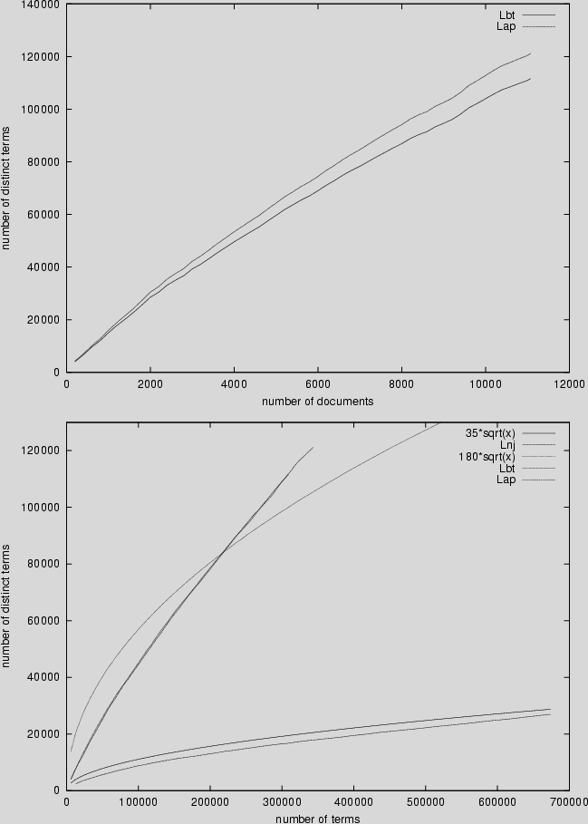
Unfortunately, binary terms did not prove more effective than adjacent pairs. That was unexpected, since the syntactically canonical nature of binary terms was thought to outperform word adjacency criteria. In a further investigation, first we measured how effective the syntactical normalization had been. Figure 3 (left) shows the comparative growth of binary terms and adjacent pairs as the dataset grows in documents.

  

Figure 3: Number of distinct terms as a function of the growing dataset (left) and as a function of the total term occurrences (right). In the right figure, two square-root curves are shown for comparison purposes. The curves of Lap and Lbt are overlapping. Obviously, the growth of composite terms cannot be approximated with a square-root.

In the whole dataset, the total distinct adjacent pairs were 121,185, while the binary terms were 111,631 (7.9% less). Clearly, our syntactical normalization had some effect, but not as extended as we expected.

How limited was the syntactical normalization is more clear in figure 3 (right). It is well-known that the number of distinct words in a growing document collection grows with the square root of the total number of word occurrences. It is obvious from this figure that this extends also to the subset of Lnj for our dataset. One could expect that the same holds for composite terms, but the number of such enriched terms grows even faster. We expected that the syntactically canonical nature of binary terms would have resulted to a less steep curve than this of adjacent pairs, but obviously it did not.