Next: 4 Parameter Estimation Up: Where to Stop Reading a Ranked List? Previous: 2 Thresholding a Ranked
Let us now elaborate on the form of the two densities ![]() and
and
![]() of Section 2.1 and their estimation.
3
of Section 2.1 and their estimation.
3
Score distributions have been modeled since the early years of IR with various known distributions [21,20,7,6]. However, the trend during the last few years, which has started in [3] and followed up in [8,1,2,14,22], has been to model score distributions by a mixture of normal-exponential densities: normal for relevant, exponential for non-relevant.
Despite its popularity, it was pointed out recently that, under a hypothesis of how systems should score and rank documents, this particular mixture of normal-exponential presents a theoretical anomaly [17]. In practice, nevertheless, it has stand the test of time in the light of
In this paper, we do not set out to investigate alternative mixtures. We theoretically extend and refine the current model in order to account for practical situations, deal with its theoretical anomaly, and improve its computation. We also check its goodness-of-fit to empirical data using a statistical test; a check that has not been done before as far as we are concerned. At the same time, we explicitly state all parameters involved, try to minimize their number, and find for them a robust set of values.
Let us consider a general retrieval model
which in theory produces scores in
![]() ,
where
,
where
![]() and
and
![]() .
By using an exponential distribution, which has semi-infinite support,
the applicability of the s-d model is restricted to those retrieval models for which
.
By using an exponential distribution, which has semi-infinite support,
the applicability of the s-d model is restricted to those retrieval models for which
![]() .
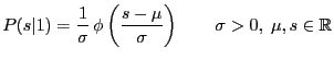
The two densities are given by
.
The two densities are given by
Over the years, two main problems of the normal-exponential model have been identified. We describe each one of them, and then introduce new models which eliminate the first problem and deal partly with the other.
From the point of view of how scores or rankings of IR systems should be, Robertson [17] formulates the recall-fallout convexity hypothesis:
For all good systems, the recall-fallout curve (as seen from [...] recall=1, fallout=0) is convex.Similar hypotheses can be formulated as a conditions on other measures, e.g., the probability of relevance should be monotonically increasing with the score; the same should hold for smoothed precision. Although, in reality, these conditions may not always be satisfied, they are expected to hold for good systems, i.e. those producing rankings satisfying the probability ranking principle (PRP), because their failure implies that systems can be easily improved.
As an example, let us consider smoothed precision. If it declines as score increases for a part of the score range, that part of the ranking can be improved by a simple random re-ordering [19]. This is equivalent of "forcing" the two underlying distributions to be uniform (i.e. have linearly increasing cdfs) in that score range. This will replace the offending part of the precision curve with a flat one--the least that can be done-- improving the overall effectiveness of the system.
Such hypotheses put restrictions on the relative forms of the two underlying distributions.
The normal-exponential mixture violates such conditions,
only (and always) at both ends of the score range.
Although the low-end scores are of insignificant importance,
the top of the ranking is very significant, especially for low ![]() topics.
The problem is a manifestation of the fact that an exponential tail
extends further than a normal one.
topics.
The problem is a manifestation of the fact that an exponential tail
extends further than a normal one.
To complicate matters further,
our data suggest that such conditions are violated at a different score ![]() for the probability of relevance and for precision.
Since the
for the probability of relevance and for precision.
Since the ![]() -measure we are interested in
is a combination of recall and precision (and recall by definition
cannot have a similar problem), we find
-measure we are interested in
is a combination of recall and precision (and recall by definition
cannot have a similar problem), we find ![]() for precision.
We force the distributions to comply with the hypothesis only when
for precision.
We force the distributions to comply with the hypothesis only when ![]() ,
where
,
where ![]() the score of the top document;
otherwise, the theoretical anomaly does not affect the score range.
If
the score of the top document;
otherwise, the theoretical anomaly does not affect the score range.
If ![]() is finite,
then two uniform distributions can be used in
is finite,
then two uniform distributions can be used in
![]() as mentioned earlier.
Alternatively, preserving a theoretical support in
as mentioned earlier.
Alternatively, preserving a theoretical support in
![]() ,
the relevant
documents distribution can be forced to an exponential in
,
the relevant
documents distribution can be forced to an exponential in
![]() with the same
with the same ![]() as this of the non-relevant.
We apply the alternative.
as this of the non-relevant.
We apply the alternative.
In fact, rankings can be further improved by reversing the offending sub-rankings; this will force the precision to increase with an increasing score, leading to better effectiveness than randomly re-ordering the sub-ranking. However, the big question here is whether the initial ranking satisfies the PRP or not. If it does, then the problem is an artifact of the normal-exponential model and reversing the sub-ranking may actually be dangerous to performance. If it does not, then the problem is inherent in the scoring formula producing the ranking. In the latter case, the normal-exponential model cannot be theoretically rejected, and it may even be used to detect the anomaly and improve rankings.
It is difficult, however, to determine whether a single ranking satisfies the PRP or not; it is well-known since the early IR years that precision for single queries is erratic, especially at early ranks, justifying the use of interpolated precision. On the one hand, according to interpolated precision all rankings satisfy the PRP, but this is forced by the interpolation. On the other hand, according to simple precision some of our rankings do not seem to satisfy the PRP, but we cannot determine this for sure. We would expect, however, that using precision averaged over all topics should produce a--more or less--declining curve with an increasing rank. Figure 1 suggests that the off-the-shelf system we currently use produces rankings that may not satisfy the PRP for ranks 5,000 to 10,000, on average.
![\includegraphics[width=4.0in]{plots/avg_estprf_rank.ps}](img113.png) |
Consequently, we rather leave open the question of whether the problem
is inherent in some scoring functions or introduced by the combined use
of normal and exponential distributions. Being conservative, we just
randomize the offending sub-rankings rather than reversing them. The
impact of this on thresholding is that the s-d method turns "blind"
inside the upper offending range; as one goes down the corresponding
ranks, precision would be flat, recall naturally rising, so the
optimal ![]() threshold can only be below the range.
threshold can only be below the range.
We will use new models that, although they do not eliminate the problem, also do not always violate such conditions imposed by the PRP (irrespective of whether it holds or not).
In order to enforce support compatibility, Arampatzis et al. [5]
introduced truncated models which we will discuss in this and the next
section. They introduced a left-truncated at ![]() normal
distribution for
normal
distribution for ![]() . With this modification, we reach a new
mixture model for score distributions with a semi-infinite support in
. With this modification, we reach a new
mixture model for score distributions with a semi-infinite support in
![]() .
.
In practice, however, scores may be naturally bounded (by the
retrieval model) or truncated to the upside as well. For example,
cosine similarity scores are naturally bounded at 1. Scores from
probabilistic models with a (theoretical) support in
![]() are usually mapped to the bounded
are usually mapped to the bounded ![]() via a
logistic function. Other retrieval models may just truncate at some maximum number
for practical reasons.
Consequently, it makes sense to introduce a right-truncation as well,
for both the normal and exponential densities.
via a
logistic function. Other retrieval models may just truncate at some maximum number
for practical reasons.
Consequently, it makes sense to introduce a right-truncation as well,
for both the normal and exponential densities.
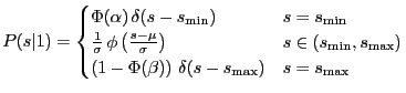
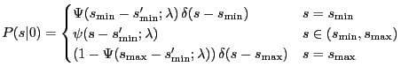
Depending on how one wants to treat the leftovers due to the truncations, two new models may be considered.
There are no leftovers (Figure 2). The underlying theoretical densities are assumed to be the truncated ones, normalized accordingly to integrate to one:
Let
![]() and
and
![]() be the random variables
corresponding to the relevant and non-relevant document
scores respectively.
The expected value and variance of
be the random variables
corresponding to the relevant and non-relevant document
scores respectively.
The expected value and variance of
![]() are given by Equations 24 and 25
in Appendix B.3.
For
are given by Equations 24 and 25
in Appendix B.3.
For
![]() ,
the corresponding Equations are
26 and 27
in Appendix B.4.
,
the corresponding Equations are
26 and 27
in Appendix B.4.
The underlying theoretical densities are not truncated, but the truncation is of a "technical" nature. The leftovers are accumulated at the two truncation points introducing discontinuities (Figure 3). For the normal, the leftovers can easily be calculated:
 |
 |
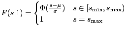
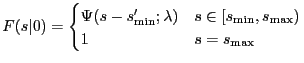
The cdfs corresponding to the above densities are:
 |
 |
The equations in this section simplify somewhat when estimating their parameters
from down-truncated ranked lists,
as we will see in Section 4.1.
We do not need to calculate ![]() .
If, for some measure, the number of non-relevant documents
is required, it can simply be estimated as
.
If, for some measure, the number of non-relevant documents
is required, it can simply be estimated as ![]() .
.
The expected values and variances of
![]() and
and
![]() ,
if needed, have to be calculated starting from
Equations 24-27
and taking into account the contribution of the discontinuities.
We do not give the formulas in this paper.
,
if needed, have to be calculated starting from
Equations 24-27
and taking into account the contribution of the discontinuities.
We do not give the formulas in this paper.
For both models the right truncation is optional.
For
![]() ,
we get
,
we get
![]() ,
leading to left-truncated models;
this accommodates retrieval models
with scoring support in
,
leading to left-truncated models;
this accommodates retrieval models
with scoring support in
![]() .
This is the maximum range that can be achieved with the current mixture,
since the restriction of a finite
.
This is the maximum range that can be achieved with the current mixture,
since the restriction of a finite ![]() is imposed by
the use of the exponential.
is imposed by
the use of the exponential.
When
![]() then
then
![]() and
and
![]() .
If additionally
.
If additionally
![]() , then
, then
![]() and
and
![]() .
Thus we can well-approximate the standard normal-exponential model.
Consequently, using a truncated model is a valid choice
even when truncations are insignificant.
.
Thus we can well-approximate the standard normal-exponential model.
Consequently, using a truncated model is a valid choice
even when truncations are insignificant.
From a theoretical point of view, it may be difficult to imagine a process producing a truncated normal directly. Truncated normal distributions are usually the results of censoring, meaning that the out-truncated data do actually exist. In this view, the technically truncated model may correspond better to the IR reality. This is also in line with the theoretical arguments for the existence of a full normal distribution [2].
Concerning convexity, both truncated models do not always violate such
conditions. Consider the problem at the top score range
![]() . In the cases of
. In the cases of
![]() , the problem is
out-truncated in both models, while--in theory--it still always
exists in the original model. The improvement so far is of a rather
theoretical nature. In practise, we should be interested in what
happens when
, the problem is
out-truncated in both models, while--in theory--it still always
exists in the original model. The improvement so far is of a rather
theoretical nature. In practise, we should be interested in what
happens when ![]() .
Our extended experiments (not reported in this paper) suggest that
truncation helps estimation in producing higher numbers of
convex fits within the observed score range. Consequently, the
benefits are also practical.
.
Our extended experiments (not reported in this paper) suggest that
truncation helps estimation in producing higher numbers of
convex fits within the observed score range. Consequently, the
benefits are also practical.
These improvements make the original model more general, and it indeed produces better fits on our data. In fact, the truncated distributions should have been used in the past during parameter estimation even for the original normal-exponential model due to down-truncated rankings.
![\includegraphics[width=4.0in]{plots/theotrunc.ps}](img120.png)
![$\displaystyle P(s\vert 1) = \frac{\frac{1}{\sigma} \, \phi \left( \frac{s-\mu} {\sigma} \right)} {\Phi(\beta) - \Phi(\alpha) } \qquad s \in [s_{\min}, s_{\max}]$](img121.png)
![$\displaystyle P(s\vert) = \frac{\psi(s-s_{\min};\lambda)} {\Psi(s_{\max}-s_{\min};\lambda)} \quad s \in [s_{\min}, s_{\max}]$](img122.png)
![\includegraphics[width=4.0in]{plots/techtrunc.ps}](img134.png)