Next: 5 Experiments Up: Where to Stop Reading a Ranked List? Previous: 3 Score Distributions
The normal-exponential mixture has worked best under the availability of some relevance judgments which serve as an indication about the form of the component densities [8,3,22]. In filtering or classification, usually some training data--although often biased--are available. In the current task, however, no relevance information is available.
A method was introduced in the context of fusion which recovers the component densities without any relevance judgments using the Expectation Maximization (EM) algorithm [14]. In order to deal with the biased training data in filtering, the EM method was also later adapted and applied for thresholding tasks [1].4 Nevertheless, EM was found to be "messy" and sensitive to its initial parameter settings [1,14]. We will improve upon this estimation method in Section 4.3.
For practical reasons, rankings are usually truncated at some rank ![]() . Even what is usually considered a full ranking is in fact a
collection's subset of those documents with at least one matching term
with the query.
. Even what is usually considered a full ranking is in fact a
collection's subset of those documents with at least one matching term
with the query.
This fact has been largely ignored in all previous research using the
standard model, despite that it may affect greatly the estimation.
For example, in TREC Legal 2007 and 2008, ![]() was
was ![]() and
and
![]() respectively. This results to a left-truncation of
respectively. This results to a left-truncation of ![]() which at least in the case of the 2007 data is significant. For 2007
it was estimated that there were more than
which at least in the case of the 2007 data is significant. For 2007
it was estimated that there were more than ![]() relevant documents
for 13 of the 43 Ad Hoc topics (to a high of more than
relevant documents
for 13 of the 43 Ad Hoc topics (to a high of more than ![]() ) and
the median system was still achieving
) and
the median system was still achieving ![]() precision at ranks of
precision at ranks of
![]() to
to ![]() .
.
Additionally, considering that the exponential may not be a good model for the whole distribution of the non-relevant scores but only for their high end, some imposed truncation may help achieve better fits. Consequently, all estimations should take place at the top of the ranking, and then get extrapolated to the whole collection. The truncated models of [5] require changes in the estimation formulas.
Let us assume that the truncation score is ![]() . For both truncated
models, we we need to estimate a two-side truncated normal at
. For both truncated
models, we we need to estimate a two-side truncated normal at ![]() and
and ![]() , and a shifted exponential by
, and a shifted exponential by ![]() right-truncated at
right-truncated at
![]() , with
, with ![]() possibly be
possibly be ![]() . Thus, the formulas
that should be used are Equations 9 and
10 but for
. Thus, the formulas
that should be used are Equations 9 and
10 but for ![]() instead of
instead of ![]()
If ![]() is the fraction of relevant documents in the truncated
ranking, extrapolating the truncated normal outside its estimation
range and appropriately per model in order to account for the
remaining relevant documents, the
is the fraction of relevant documents in the truncated
ranking, extrapolating the truncated normal outside its estimation
range and appropriately per model in order to account for the
remaining relevant documents, the ![]() is calculated as:
is calculated as:
In estimating
the technically truncated model,
if there are any scores equal to ![]() or
or ![]() they should be removed from the data-set;
these belong to the discontinuous legs of
the densities given in Section 3.3.2.
In this case,
they should be removed from the data-set;
these belong to the discontinuous legs of
the densities given in Section 3.3.2.
In this case, ![]() should be decremented accordingly.
In practise, while scores equal to
should be decremented accordingly.
In practise, while scores equal to
![]() should not exist in the top-
should not exist in the top-![]() due to the
down-truncation, some
due to the
down-truncation, some ![]() scores may very well be in the
data. Removing these during estimation is a simplifing
approximation with an insignificant impact when the relevant
documents are many and the bulk of their score distribution is below
scores may very well be in the
data. Removing these during estimation is a simplifing
approximation with an insignificant impact when the relevant
documents are many and the bulk of their score distribution is below
![]() , as it is the case in current experimental setup. As we
will see next, while we do not use the
, as it is the case in current experimental setup. As we
will see next, while we do not use the ![]() scores during
fitting, we take them into account during goodness-of-fit testing;
using multiple such fitting/testing rounds, this reduces the impact
of the approximation.
scores during
fitting, we take them into account during goodness-of-fit testing;
using multiple such fitting/testing rounds, this reduces the impact
of the approximation.
Our scores have a resolution of ![]() . Obviously, LUCENE
rounds or truncates the output scores, destroying information. In
order to smooth out the effect of rounding in the data, we add
. Obviously, LUCENE
rounds or truncates the output scores, destroying information. In
order to smooth out the effect of rounding in the data, we add
![]() to each datum point, where
to each datum point, where
![]() returns a uniformly-distributed real random number
in
returns a uniformly-distributed real random number
in ![]() .
.
Beyond using all scores available and in order to speed up the calculations, we also tried stratified down-sampling to keep only 1 out of 2, 3, or 10 scores.5Before any down-sampling, all datum points were smoothed by replacing them with their average value in a surrounding window of 2, 3, or 10 points, respectively.
In order to obtain better exponential fits we may further left-truncate the rankings at the mode of the observed distribution. We bin the scores (as described in Section A.1), find the bin with the most scores, and if that is not the leftmost bin then we remove all scores in previous bins.
EM is an iterative procedure which converges locally [9]. Finding a global fit depends largely on the initial settings of the parameters.
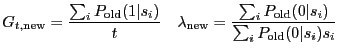
We tried numerous initial settings, but no setting seemed universal. While some settings helped a lot some fits, they had a negative impact on others. Without any indication of the form, location, and weighting of the component densities, the best fits overall were obtained for randomized initial values, preserving also the generality of the approach:6
where
Assuming that no information is available about the expected ![]() ,
not much can be done for
,
not much can be done for
![]() ,
so it is randomized using its whole supported range.
Next
we assume that right-truncation of the exponential
is insignificant, which seems to be the case in our current experimental set-up.
,
so it is randomized using its whole supported range.
Next
we assume that right-truncation of the exponential
is insignificant, which seems to be the case in our current experimental set-up.
If there are no relevant documents, then
![]() .
From the last equation we deduce the minimum
.
From the last equation we deduce the minimum
![]() .
Although in general, there is no reason why the exponential
cannot fall slower that this, from an IR perspective it should not,
or
.
Although in general, there is no reason why the exponential
cannot fall slower that this, from an IR perspective it should not,
or
![]() would get higher than
would get higher than
![]() .
.
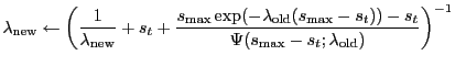
The
![]() given is suitable for a full normal, and its range
should be expanded in both sides for a truncated one because the mean
of the corresponding full normal can be below
given is suitable for a full normal, and its range
should be expanded in both sides for a truncated one because the mean
of the corresponding full normal can be below ![]() or above
or above
![]() . Further,
. Further,
![]() can be restricted based on the hypothesis
that for good systems should hold that
can be restricted based on the hypothesis
that for good systems should hold that
![]() . We have not worked out these improvements.
. We have not worked out these improvements.
The variance of the initial exponential is
![]() .
Assuming that the random variables corresponding to the normal and exponential
are uncorrelated, the variance of the normal is
.
Assuming that the random variables corresponding to the normal and exponential
are uncorrelated, the variance of the normal is
![]() which, depending on how
which, depending on how ![]() is initialized,
could take values
is initialized,
could take values ![]() . To avoid this, we take the max with the constant.
For an insignificantly truncated normal,
. To avoid this, we take the max with the constant.
For an insignificantly truncated normal,
![]() , while in general
, while in general ![]() ,
because the variance of the corresponding full normal is larger than what is
observed in the truncated data. We set
,
because the variance of the corresponding full normal is larger than what is
observed in the truncated data. We set ![]() , however, we found its usable range
to be
, however, we found its usable range
to be ![]() .
.
For ![]() observed scores
observed scores
![]() ,
and neither truncated nor shifted normal and exponential densities
(i.e. for the original model),
the update equations are
,
and neither truncated nor shifted normal and exponential densities
(i.e. for the original model),
the update equations are

We initialize those equations as described above,
and iterate them until the absolute differences between
the old and new values for ![]() ,
,
![]() , and
, and
![]() are all less than
are all less than
![]() , and
, and
![]() . Like this we target an accuracy of 0.1% for
scores and 1 in a 1,000 for documents.
We also tried a target accuracy of 0.5% and 5 in 1,000,
but it did not seem sufficient.
. Like this we target an accuracy of 0.1% for
scores and 1 in a 1,000 for documents.
We also tried a target accuracy of 0.5% and 5 in 1,000,
but it did not seem sufficient.
If we use the truncated densities
(Equations 9 and 10)
in the above update equations,
the
![]() and
and
![]() calculated at each iteration would be
the expected value and variance of the truncated normal,
not the
calculated at each iteration would be
the expected value and variance of the truncated normal,
not the ![]() and
and ![]() we are looking for.
Similarly,
we are looking for.
Similarly,
![]() would be equal to
the expected value of the shifted truncated exponential.
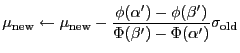
Instead of looking for new EM equations, we rather correct to the right values
using simple approximations.
would be equal to
the expected value of the shifted truncated exponential.
Instead of looking for new EM equations, we rather correct to the right values
using simple approximations.
Using Equation 26,
at the end of each iteration we correct the calculated
![]() as
as
again using the values from the previous iteration.
These simple approximations work, but sometimes they seem to increase the number of iterations needed for convergence, depending on the accuracy targeted. Rarely, and for high accuracies only, the approximations possibly handicap EM convergence; the intended accuracy is not reached for up to 1,000 iterations. Generally, convergence happens in 10 to 50 iterations depending on the number of scores (more data, slower convergence), and even with the approximation EM produces considerably better fits than when using the non-truncated densities. To avoid getting locked in a non-converging loop, despite its rarity, we cap the number of iterations to 100. The end-differences we have seen between the observed and expected numbers of documents due to these approximations have always been less than 4 in 100,000.
We initialize and run EM as described above.
After EM stops,
we apply the ![]() goodness-of-fit test
for the observed data and the recovered mixture (see Appendix A).
If the null hypothesis
goodness-of-fit test
for the observed data and the recovered mixture (see Appendix A).
If the null hypothesis
![]() is rejected, we randomize again the initial values and repeat EM for up to 100 times
or until
is rejected, we randomize again the initial values and repeat EM for up to 100 times
or until
![]() cannot be rejected.
If
cannot be rejected.
If
![]() is rejected in all 100 runs,
we just keep the best fit found.
We run EM at least 10 times, even if we cannot reject
is rejected in all 100 runs,
we just keep the best fit found.
We run EM at least 10 times, even if we cannot reject
![]() earlier.
Perhaps a maximum of 100 EM runs is an overkill,
but we found that there is significant sensitivity to initial conditions.
earlier.
Perhaps a maximum of 100 EM runs is an overkill,
but we found that there is significant sensitivity to initial conditions.
Some fits, irrespective of their quality, can be rejected on IR grounds.
Firstly,
it should hold that ![]() , however,
since each fit corresponds to
, however,
since each fit corresponds to
![]() non-relevant documents,
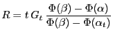
we can tighten the inequality somewhat to:
non-relevant documents,
we can tighten the inequality somewhat to:
| (15) |
| run |
|
|
|
|
|
|
comments |
| 2007-default | 56.5 | 4 (8%) | 2 (4%) | 33 (66%) | 29 | 5 (10%) | no smth or sampling |
| 2007-A | 37 | 1 (2%) | 32 (64%) | 40 (80%) | 34 | 5 (10%) | smth + 1/3 strat. sampl. |
| 2007-B | 36 | 1 (2%) | 30 (60%) | 32 (64%) | 61.5 | 1 (2%) | smth + 1/3 strat. sampl. |
| 2008-default | 93 | 6 (13%) | 0 (0%) | 29 (64%) | 89 | 0 (0%) | no smth or sampling |
| 2008-A | 63 | 1 (2%) | 5 (11%) | 30 (67%) | 98 | 0 (0%) | smth + 1/3 strat. sampl. |
| 2008-B | 66 | 4 (9%) | 9 (20%) | 31 (69%) | 45 | 1 (2%) | smth +1/3 strat. sampl. |
We are still experimenting with such conditions, and we have not applied them for producing any of the end-results reported in this paper.
Down-sampling has the effect of eliminating some of the right tails,
leading to fewer bins when binning the data. Moreover, the fewer the
scores, the less EM iterations and runs are needed for a good fit
(data not shown). Down-sampling the scores helps supporting the
![]() . At 1 out of 3 stratified sampling, the
. At 1 out of 3 stratified sampling, the
![]() cannot be rejected at a significance level of 0.05 for 60-64% of the
2007 topics and for 20% for the 2008 topics. Non-stratified
down-sampling with 0.1 probability raises this to 42% for the 2008
topics. Extreme down-sampling to keep only around 1,000 to 5,000
scores supports the
cannot be rejected at a significance level of 0.05 for 60-64% of the
2007 topics and for 20% for the 2008 topics. Non-stratified
down-sampling with 0.1 probability raises this to 42% for the 2008
topics. Extreme down-sampling to keep only around 1,000 to 5,000
scores supports the
![]() in almost all fits.
in almost all fits.
Consequently, the number of scores and bins plays a big role in the
quality of the fits according to the ![]() test; there is a
positive correlation between the median number of bins
test; there is a
positive correlation between the median number of bins
![]() and the percentage of rejected
and the percentage of rejected
![]() . This effect does not
seem to be the result of information loss due to down-sampling; we
still get more support for the
. This effect does not
seem to be the result of information loss due to down-sampling; we
still get more support for the
![]() when reducing the number
of scores by down-truncating the rankings instead of down-sampling
them. This is an unexpected result; we rather expected that the
increased number of scores and bins is dealt with by the increased
degrees of freedom parameter of the corresponding
when reducing the number
of scores by down-truncating the rankings instead of down-sampling
them. This is an unexpected result; we rather expected that the
increased number of scores and bins is dealt with by the increased
degrees of freedom parameter of the corresponding ![]() distributions. Irrespective of sampling and binning, however, all
fits look reasonably well to the eye.
distributions. Irrespective of sampling and binning, however, all
fits look reasonably well to the eye.
In all runs, for a small fraction of topics (2-13%) the optimum
number of bins ![]() is near (
is near (![]() difference) to our capped value of
200. For most of these topics, when looking for the optimal number of
bins in the range
difference) to our capped value of
200. For most of these topics, when looking for the optimal number of
bins in the range ![]() (numbers are tried with a step of 5%)
the binning method does not converge. This means there is no optimal
binning as the algorithm identifies the discrete structure of data as
being a more salient feature than the overall shape of the density
function. Figure 4 demonstrates this.
(numbers are tried with a step of 5%)
the binning method does not converge. This means there is no optimal
binning as the algorithm identifies the discrete structure of data as
being a more salient feature than the overall shape of the density
function. Figure 4 demonstrates this.
![\includegraphics[width=4.0in]{plots/73.ps}](img295.png) |
Since the scores are already randomized to account for rounding (Section 4.2), the discrete structure of the data is not a result of rounding but it rather comes from the retrieval model itself. Internal statistics are usually based on document and word counts; when these are low, statistics are "rough", introducing the discretization effect.
Concerning the theoretical anomaly of the normal-exponential mixture,
we investigate the number of fits presenting the anomaly within the
observed score range, i.e. at a rank below rank-1 (![]() ).7 We see that the
anomaly shows up in a large number of topics (64-80%). The impact of
non-convexity on the s-d method is that the method turns "blind" at
rank numbers
).7 We see that the
anomaly shows up in a large number of topics (64-80%). The impact of
non-convexity on the s-d method is that the method turns "blind" at
rank numbers ![]() restricting the estimated optimal thresholds wtih
restricting the estimated optimal thresholds wtih
![]() . However, the median rank number
. However, the median rank number
![]() down
to which the problem exists is very low compared to the median
estimated number of relevant documents
down
to which the problem exists is very low compared to the median
estimated number of relevant documents
![]() (7,484 or
32,233), so
(7,484 or
32,233), so ![]() is unlikely on average anyway and thresholding
should not be affected.
Consequently, the data suggest that the non-convexity should have an
insignificant impact on s-d thresholding.
is unlikely on average anyway and thresholding
should not be affected.
Consequently, the data suggest that the non-convexity should have an
insignificant impact on s-d thresholding.
For a small number of topics (0-10%), the problem appears for
![]() and non-convexity should have a significant impact.
Still, we argue that for a good fraction of such topics, a large
and non-convexity should have a significant impact.
Still, we argue that for a good fraction of such topics, a large ![]() indicates a fitting problem rather than a theoretical one.
Figure 5 explains this further.
indicates a fitting problem rather than a theoretical one.
Figure 5 explains this further.
![\includegraphics[width=4.0in]{plots/91.ps}](img308.png)
![\includegraphics[width=4.0in]{plots/91R2.ps}](img309.png) |
Since there are more data at lower scores, EM results in parameter
estimates that fit the low scores better than the high scores. This
is exactly the opposite of what is needed for IR purposes, where the
top of rankings is more important. It also introduces a weak but
undesirable bias: the longer the input ranked list, the lower the
estimates of the means of the normal and exponential; this usually
results in larger estimations of ![]() and
and ![]() .
.
Trying to neutralize the bias without actually removing it, input
ranking lengths can better be chosen according to the expected ![]() .
This also makes sense for the estimation method irrespective of
biases: we should not expect much when trying to estimate, e.g., an
.
This also makes sense for the estimation method irrespective of
biases: we should not expect much when trying to estimate, e.g., an
![]() of 100,000 from only the top-1000. As a rule-of-thumb, we
recommend input ranking lengths of around 1.5 times the expected
of 100,000 from only the top-1000. As a rule-of-thumb, we
recommend input ranking lengths of around 1.5 times the expected ![]() with a minimum of 200.
According to this recommendation, the 2007 rankings truncated at
25,000 are spot on, but the 100,000 rankings of 2008 are falling short
by 20%.
with a minimum of 200.
According to this recommendation, the 2007 rankings truncated at
25,000 are spot on, but the 100,000 rankings of 2008 are falling short
by 20%.
Recovering the mixture with EM has been proven to be "tricky". However, with the improvements presented in this paper, we have reached a rather stable behavior which produces usable fits.
EM's initial parameter settings can further be tightened resulting in better estimates in less iterations and runs, but we have rather been conservative in order to preserve the generality.
As a result of how EM works--giving all data equal importance--a
weak but undesirable ranking-length bias is present: the longer the
input ranking, the larger the ![]() estimates. Although the problem can
for now be neutralized by choosing the input lengths in accordance
with the expected
estimates. Although the problem can
for now be neutralized by choosing the input lengths in accordance
with the expected ![]() , any future improvements of the estimation
method should take into account that score data are of unequal
importance:
data should be fitted better at their high end.
, any future improvements of the estimation
method should take into account that score data are of unequal
importance:
data should be fitted better at their high end.
Whatever the estimation method, conditions for rejecting fits on IR grounds such as those investigated in Section 4.3.5, seem to have a potential for further considerable improvements.
![$\displaystyle \sigma_\mathrm{new}^2 \leftarrow \sigma_\mathrm{new}^2 \left[ 1 +...
...(\alpha') - \phi(\beta')} {\Phi(\beta') - \Phi(\alpha')} \right)^2 \right]^{-1}$](img257.png)